simdkalman documentation

Fast Kalman filters in Python leveraging single-instruction multiple-data vectorization. That is, running n similar Kalman filters on n independent series of observations. Not to be confused with SIMD processor instructions.

See full documentation.

Installation: pip install simdkalman

Source code: https://github.com/oseiskar/simdkalman

License: MIT

Terminology

Following the notation in [1], the Kalman filter framework consists of a dynamic model (state transition model)

\[x_k = A x_{k-1} + q_{k-1}, \qquad q_{k-1} \sim N(0, Q)\]

and a measurement model (observation model)

\[y_k = H x_k + r_k, \qquad r_k \sim N(0, R),\]

where the vector \(x\) is the (hidden) state of the system and \(y\) is an observation. A and H are matrices of suitable shape and \(Q\), \(R\) are positive-definite noise covariance matrices.

[1]

Simo Sarkkä (2013). Bayesian Filtering and Smoothing. Cambridge University Press. https://users.aalto.fi/~ssarkka/pub/cup_book_online_20131111.pdf

Usage example

Define model

import simdkalman
import numpy as np

kf = simdkalman.KalmanFilter(
    state_transition = [[1,1],[0,1]],        # matrix A
    process_noise = np.diag([0.1, 0.01]),    # Q
    observation_model = np.array([[1,0]]),   # H
    observation_noise = 1.0)                 # R

Generate some fake data

import numpy.random as random

# 100 independent time series
data = random.normal(size=(100, 200))

# with 10% of NaNs denoting missing values
data[random.uniform(size=data.shape) < 0.1] = np.nan

Smooth all data

smoothed = kf.smooth(data,
                     initial_value = [1,0],
                     initial_covariance = np.eye(2) * 0.5)

# second timeseries, third time step, hidden state x
print('mean')
print(smoothed.states.mean[1,2,:])

print('covariance')
print(smoothed.states.cov[1,2,:,:])

mean
[ 0.29311384 -0.06948961]
covariance
[[ 0.19959416 -0.00777587]
 [-0.00777587  0.02528967]]

Predict new data for a single series (1d case)

predicted = kf.predict(data[1,:], 123)

# predicted observation y, third new time step
pred_mean = predicted.observations.mean[2]
pred_stdev = np.sqrt(predicted.observations.cov[2])

print('%g +- %g' % (pred_mean, pred_stdev))

1.71543 +- 1.65322

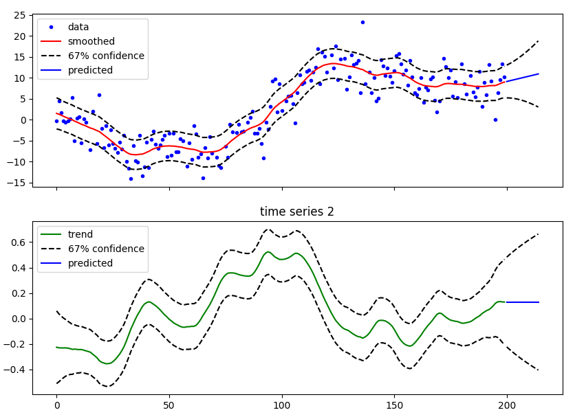
For complete code examples with figures, see: https://github.com/oseiskar/simdkalman/blob/master/examples/ and this Gist.

Usage of multi-dimensional observations is demonstrated in this example.

Extended Kalman Filters (EKF) can be implemented using the simdkalman.primitives module, see example.

Class documentation

class simdkalman.KalmanFilter(state_transition, process_noise, observation_model, observation_noise)

The main Kalman filter class providing convenient interfaces to vectorized smoothing and filtering operations on multiple independent time series.

As long as the shapes of the given parameters match reasonably according to the rules of matrix multiplication, this class is flexible in their exact nature accepting

• scalars: process_noise = 0.1

• (2d) numpy matrices: process_noise = numpy.eye(2)

• 2d arrays: observation_model = [[1,2]]

• 3d arrays and matrices for vectorized computations. Unlike the other options, this locks the shape of the inputs that can be processed by the smoothing and prediction methods.

Parameters:

• state_transition – State transition matrix \(A\)

• process_noise – Process noise (state transition covariance) matrix \(Q\)

• observation_model – Observation model (measurement model) matrix \(H\)

• observation_noise – Observation noise (measurement noise covariance) matrix \(R\)

compute(data, n_test, initial_value=None, initial_covariance=None, smoothed=True, filtered=False, states=True, covariances=True, observations=True, likelihoods=False, gains=False, log_likelihood=False, verbose=False)

Smoothing, filtering and prediction at the same time. Used internally by other methods, but can also be used directly if, e.g., both smoothed and predicted data is wanted.

See smooth and predict for explanation of the common parameters. With this method, there also exist the following flags.

Parameters:

• smoothed (boolean) – compute Kalman smoother (used by smooth)

• filtered (boolean) – return (one-way) filtered data

• likelihoods (boolean) – return likelihoods of each step

• gains (boolean) – return Kalman gains and pairwise covariances (used by the EM algorithm). If true, the gains are provided as a member of the relevant subresult filtered.gains and/or smoothed.gains.

• log_likelihood (boolean) – return the log-likelihood(s) for the entire series. If matrix data is given, this will be a vector where each element is the log-likelihood of a single row.

Return type:

result object whose fields depend on of the above parameter flags are True. The possible values are: smoothed (the return value of smooth, may contain smoothed.gains), filtered (like smoothed, may also contain filtered.gains), predicted (the return value of predict if n_test > 0) pairwise_covariances, likelihoods and log_likelihood.

predict(data, n_test, initial_value=None, initial_covariance=None, states=True, observations=True, covariances=True, verbose=False)

Filter past data and predict a given number of future values. The data can be given as either of

• 1d array, like [1,2,3,4]. In this case, one Kalman filter is used and the return value structure will contain an 1d array of observations (both .mean and .cov will be 1d).

• 2d matrix, whose each row is interpreted as an independent time series, all of which are filtered independently. The returned observations members will be 2-dimensional in this case.

• 3d matrix, whose the last dimension can be used for multi-dimensional observations, i.e, data[1,2,:] defines the components of the third observation of the second series. In the-multi-dimensional case the returned observations.mean will be 3-dimensional and observations.cov 4-dimensional.

Initial values and covariances can be given as scalars or 2d matrices in which case the same initial states will be used for all rows or 3d arrays for different initial values.

Parameters:

• data – Past data

• n_test (integer) – number of future steps to predict.

• initial_value – Initial value \({\mathbb E}[x_0]\)

• initial_covariance – Initial uncertainty \({\rm Cov}[x_0]\)

• states (boolean) – predict states \(x\)?

• observations (boolean) – predict observations \(y\)?

• covariances (boolean) – include covariances in predictions?

Return type:

Result object with fields states and observations, if the respective parameter flags are set to True. Both are Gaussian result objects with fields mean and cov (if the covariances flag is True)

predict_next(m, P)

Single prediction step

Parameters:

• m – \({\mathbb E}[x_{j-1}]\), the previous mean

• P – \({\rm Cov}[x_{j-1}]\), the previous covariance

Return type:

(prior_mean, prior_cov) predicted mean and covariance \({\mathbb E}[x_j]\), \({\rm Cov}[x_j]\)

predict_observation(m, P)

Probability distribution of observation \(y\) for a given distribution of \(x\)

Parameters:

• m – \({\mathbb E}[x]\)

• P – \({\rm Cov}[x]\)

Return type:

mean \({\mathbb E}[y]\) and covariance \({\rm Cov}[y]\)

smooth(data, initial_value=None, initial_covariance=None, observations=True, states=True, covariances=True, verbose=False)

Smooth given data, which can be either

• 1d array, like [1,2,3,4]. In this case, one Kalman filter is used and the return value structure will contain an 1d array of observations (both .mean and .cov will be 1d).

• 2d matrix, whose each row is interpreted as an independent time series, all of which are smoothed independently. The returned observations members will be 2-dimensional in this case.

• 3d matrix, whose the last dimension can be used for multi-dimensional observations, i.e, data[1,2,:] defines the components of the third observation of the second series. In the-multi-dimensional case the returned observations.mean will be 3-dimensional and observations.cov 4-dimensional.

Initial values and covariances can be given as scalars or 2d matrices in which case the same initial states will be used for all rows or 3d arrays for different initial values.

Parameters:

• data – 1d or 2d data, see above

• initial_value – Initial value \({\mathbb E}[x_0]\)

• initial_covariance – Initial uncertainty \({\rm Cov}[x_0]\)

• states (boolean) – return smoothed states \(x\)?

• observations (boolean) – return smoothed observations \(y\)?

• covariances (boolean) – include covariances results? For lower memory usage, set this flag to False.

Return type:

Result object with fields states and observations, if the respective parameter flags are set to True. Both are Gaussian result objects with fields mean and cov (if the covariances flag is True)

smooth_current(m, P, ms, Ps)

Simgle Kalman smoother backwards step

Parameters:

• m – \({\mathbb E}[x_j|y_1,\ldots,y_j]\), the filtered mean of \(x_j\)

• P – \({\rm Cov}[x_j|y_1,\ldots,y_j]\), the filtered covariance of \(x_j\)

• ms – \({\mathbb E}[x_{j+1}|y_1,\ldots,y_T]\)

• Ps – \({\rm Cov}[x_{j+1}|y_1,\ldots,y_T]\)

Return type:

(smooth_mean, smooth_covariance, smoothing_gain) smoothed mean \({\mathbb E}[x_j|y_1,\ldots,y_T]\), and covariance \({\rm Cov}[x_j|y_1,\ldots,y_T]\) & smoothing gain \(C\)

update(m, P, y, log_likelihood=False)

Single update step with NaN check.

Parameters:

• m – \({\mathbb E}[x_j|y_1,\ldots,y_{j-1}]\), the prior mean of \(x_j\)

• P – \({\rm Cov}[x_j|y_1,\ldots,y_{j-1}]\), the prior covariance of \(x_j\)

• y – observation \(y_j\)

• log_likelihood – compute log-likelihood?

Return type:

(posterior_mean, posterior_covariance, log_likelihood) posterior mean \({\mathbb E}[x_j|y_1,\ldots,y_j]\) & covariance \({\rm Cov}[x_j|y_1,\ldots,y_j]\) and, if requested, log-likelihood. If \(y_j\) is NaN, returns the prior mean and covariance instead

Primitives

The simdkalman.primitives module contains low-level Kalman filter computation steps with multi-dimensional input arrays. See this page for full documentation.

Change log

See https://github.com/oseiskar/simdkalman/releases